Ch 8: CCSM Measures for Thermal Storage Systems
Thermal storage systems are intended to meet part or all of the cooling needs of a building during specified periods of peak demand. It is essential they have sufficient capacity to provide the cooling during these periods. Figure 8-1 presents the schematic diagram of a thermal storage system. During off-peak hours, part of the cooling energy produced by the chillers is used for charging the storage systems that generally store cold water or ice. During peak hours, buildings receive cooling energy from the tank and/or chillers.
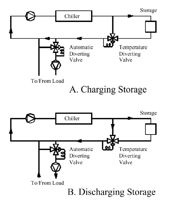
Figure 8-1. Thermal Storage System in Charging Mode and in Discharge Mode
Thermal storage systems save costs by decreasing peak electrical demand during the electric utility’s peak demand window. However, the billed demand may also depend on off-peak demand. Therefore, the cost savings strongly depend on the utility rate structure. For example, if there is a ratchet on the demand, a single system failure during the summer peak can largely eliminate the savings produced by the system for the entire year. Although optimizing thermal storage operation often requires special considerations based on each case, several CCSM measures apply to any type of thermal storage system. This chapter only discusses these measures.
8.1 Maximize Building Return Water Temperature
Low return water temperature is the primary problem with thermal storage systems. A low return water temperature prevents the chiller from operating at full load. Consequently, the chiller may not be able to charge the tank during off-peak hours. A low return water temperature can also significantly reduce the storage capacity of the system. For example, if the building return temperature is 50°F instead of 54°F, the thermal storage capacity will be decreased by 33% if the design temperature difference is 12°F. To increase the return water temperature, the following procedures should be followed:
Implement building loop and secondary loop CCSM measures. The key measures are repeated below:
- Close three-way valves on the cooling coils
- Close building by-pass to prevent supply water from flowing directly back to the plant
- Optimize building loop and secondary loop differential pressure set points
- Ensure supply air temperatures are set properly and control valves are functioning properly. Any excessively low supply air temperature set points can cause low return water temperatures. For example, setting the air temperature at 50°F instead of 55°F will cause the control valve to open fully if the chilled water supply temperature is 42°F. The return temperature will be well below 54°F.
Use a blending station to control return water temperature if the building water balance problems cannot be solved in a timely manner. This blends part of the building return water with primary cooling water before sending it to the building. Using the blending station causes extra pump power consumption and may also cause humidity control problems. As soon as the water balance is improved, the blending station should be disabled.
8.2 Improve Chilled Water Flow Control Through Chillers
It is important to control the chilled water flow at the design value. If the chilled water flow is lower than design flow, the chiller will not be able to produce full capacity. The tank may not be fully charged as a result. If the chilled water flow is higher than the design flow value, the chilled water supply temperature will not control at the required value. The tank capacity can be decreased significantly. For example, if the chilled water supply temperature is 44°F instead of 42°F, the tank capacity is decreased by 16% based on a design temperature difference of 12°F. To improve the chilled water flow control through chillers, the following guidelines are given:
- If cooling is not provided to the building at night, the designated loop config- uration should be determined. Balance the system to allow design chilled water flow through chillers and tanks at night.
- If cooling is required at night, use a lower loop differential pressure set point for the building loop at night. Reset cold air supply temperature to a higher value if that is acceptable.
- Modulate tank charging pump to maintain a constant chilled water flow through the chiller. This requires special handling on a case by case basis.
EXAMPLE:
A thermal storage system was installed in a 37,000 sq.ft. county hospital in Monahans, Texas, in the early 1990s. The hospital has a 120-ton chiller and the thermal storage system included a 80,675 gallon above ground chilled water storage tank shown in Figure 8-2.
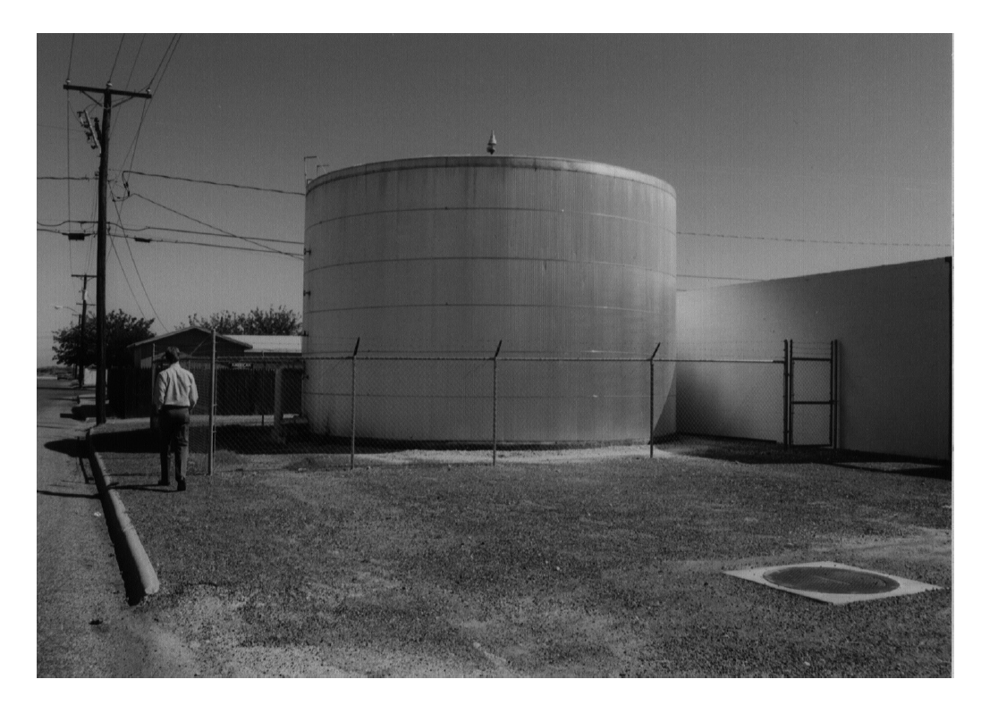
Figure 8-2. Chilled Water Storage Tank at the Hospital in Monahans, Texas
The waterside of the chiller/thermal storage system is shown in Figure 8-3. The figure shows the system in the tank discharge mode with the chiller isolated from the loop. The tank pump shown has a 125 gpm capacity, while the design flow rate in the building loop is 180 gpm. The chiller pump capacity is 228 gpm. The building has 12 small roof top units to serve the administrative areas. Two control valves are used for the cooling coil. The patient rooms were conditioned by 32 fan-coil units connected to the chilled water loop through three way valves.
The thermal storage system had problems from the beginning and appeared to have inadequate storage capacity, and/or chiller capacity, to handle the cooling requirements of the hospital during the noon to 8 p.m. peak window. The chiller had to be brought on during some of the hottest days. Figure 8-4 presents the hourly whole building electricity consumption of the hospital plotted from midnight on the left through the 24 hours of one day on the right. The first line visible at the front of the figure is the data for July 31. The second line the data for July 30, etc., with two months of data shown in the figure. The figure shows that on July 31, consumption through the early hours of the morning was somewhat above 200 kW, rising above 250 kW by noon, and dropping to levels near 100 kW until around 8:00 p.m. when it increased to about 200 kW. Hence, the thermal storage system had operated properly and the chiller had not been operated during the peak demand window from noon to 8 p.m. However, many days are visible when the chiller operated during this window. The days when the chiller operated continuously were generally weekend days when there was no penalty for operation during this period. The operators were trying to get the storage fully charged so they would be able to handle the loads during the week. However, several lines are visible where it appears the chiller went off, then came back on in the late afternoon. In these cases the system was not operating as designed.
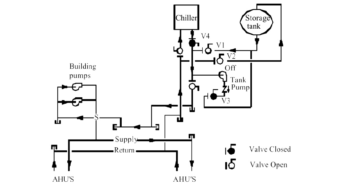
Figure 8-3. Waterside Schematic of the Chiller/Thermal Storage System at the Hospital in Monahans, Texas
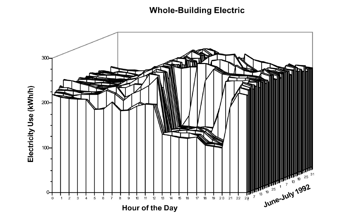
Figure 8-4. Hourly Electricity Consumption for the Hospital in Monahans, Texas, for June and July, 1993
Field measurements identified the following problems:
- The highest differential temperature in the building loop was 7°F (42/49°F), which indicates the building loop flow was at least 70% higher than required. The low differential temperature was largely due to chilled water bypass of the fan coils and a few coils in the roof top units, where excessive outside air was used.
- Measurements showed the chilled water flow to the building reached 200 gpm. Since the chiller rated flow rate is 228 gpm, the chilled water flow to the tank was much lower than the tank pump capacity of 128 gpm and the tank could not be fully charged during the off-peak hours.
To solve the problem, the following actions were taken:
Conducted AHU system commissioning, which included the following major items:
- Decreased outside air intake by up to 50% in five major roof top units. Since no return air fan was installed, the mixed air chamber had a negative pressure of –1.0 in. H2O or lower. The negative pressure sucked excessive outside air into the AHU. However, the cooling coil did not have the capacity to handle the outside air. This caused the cooling control valve to fully open. Reducing the outside air flow to the required level allows the chilled water control valve to function properly. Eliminating the three-way valves was not immediately implemented due to lack of funds for that purpose.
- Calibrated the cold air temperature sensor and set the supply air temperature at a minimum of 55°F
Installed a VFD on the building pump and a temperature sensor on both the return and supply.
- Modulated VFD speed to control the differential temperature at a minimum of 10°F. The differential pressure sensor was not used since the system did not include a differential pressure sensor and funds were not available for installation.
- Set the maximum VFD speed to 60%. There was no manual valve in the bypass line of the fan coil unit. It was also impossible to cut off the bypass line when the system was commissioned. However, engineering calculations showed that the three-way valve would be 90% open to the coil if the VFD was set at 60% under maximum building load conditions. Although this does not maximize the pump power savings, it would provide reliable system operation. This was the top priority of the project.
Figure 8-5 shows the building electricity consumption during June and July the summer after these measures were implemented. It can be seen that it was never necessary to operate the chiller during the peak demand window. The system has operated successfully through some of the hottest summers in Texas history since then.
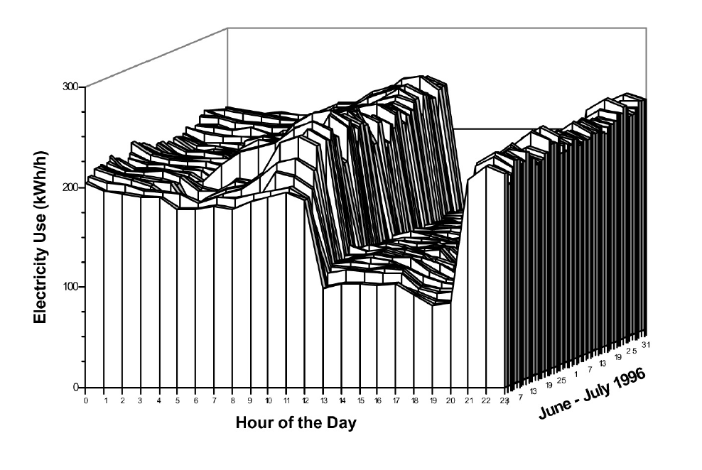
Figure 8-5. Electricity Consumption for Hospital in Monahans Texas Following Implementation of CCSM Measures
The pump power before and after the CC process is shown in Figure 8-6. The pumping power has typically been reduced by 50% or more.
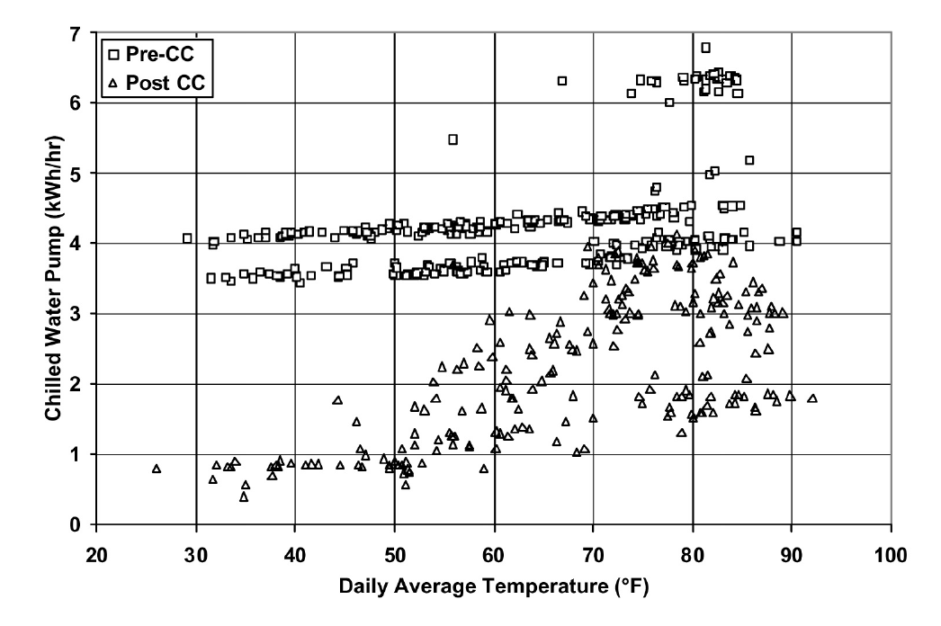
Figure 8-6. Pumping Power at the Monahans, Texas, Hospital Before and After CCSM Measures Were Implemented
The savings from restoring the thermal storage system to operation were $14,190/year, with additional savings of $5,540/year resulting from the improved pump and AHU operation, for total savings of $19,730/yr. More information can be found in “Rehabilitating a Thermal Storage System through Commissioning” [Liu et al. 1999].
8.3 Minimize the Off-Peak Demand
Some utility rate schedules also use off-peak demand to determine the billing demand. In these cases, decreasing off-peak demand can also result in significant cost savings. To decrease the off-peak demand, the following procedures should be followed:
- Turn off the chiller earlier. If the peak period starts at noon, the off-peak demand is often set between 10:00 a.m. and noon. Turning off one or two chillers during this short period can result in significant off-peak demand reduction.
- Turn on chiller earlier. If the peak period ends after 6:00 p.m., one or more chillers can often be turned on after 5:00 p.m. since office lights and equipment are gradually turned off beginning at 5:00 p.m. or even earlier. Turn on one or more chillers to keep a constant peak demand over the off-peak period.
- Do not entirely charge the tank in a single day when cooling requirements are low. During mild days or during the winter, a small amount of cooling may be required. The tank should be partially charged to minimize the thermal losses. The tank should not be fully charged in a single day since it may require turning on all chillers for a short period and could set up a very high off-peak demand for that month.
EXAMPLE:
Terrell State Hospital, located in Terrell, Texas, is a mental health campus with more than 600,000 square feet of conditioned space in more than a dozen buildings. A chilled water thermal storage system with 7,000 ton-hours capacity was constructed in 1995 to provide cooling to the campus. There are four chillers in three different chiller plants, with total cooling capacity of 1,325 tons (two 425-ton, one 275-ton and one 200-ton).
On-peak hours were from noon to 8:00 p.m. weekdays, June through September. The thermal storage system was intended to decrease on-peak demand by 700 kW. Figure 8-7 presents the procedures for determining billed demand. First, demand candidate 1 was determined as the lesser of the current month’s peak demand (off-peak or on-peak) and as a factor including ratchet demand and current off-peak demand (25% current off-peak demand plus 75% of the highest on-peak demand in the last 12 months). Secondly, demand candidate 2 was determined as the largest of the following: (1) a ratchet factor, 80% of the annual on-peak demand, (2) 50% of the contract demand and (3) 50% of the annual peak demand, including off-peak demand. The actual monthly demand charge was based on the larger of the two candidate values.
The hospital had a contract demand of 2,800 kW meaning it had a 1,400 kW minimum monthly demand charge. The peak demand hours were from noon to 8:00 p.m., Monday through Friday during the months of June, July, August and September. The historical on-peak demand varied from 1,475 kW to 1,731 kW during the on-peak months. The off-peak demand varied from 1,678 kW to 2,736 kW. Figure 8-8 presents the simulated demand penalties with hypothetical on-peak demand and off-peak demand values. The demand penalty is defined as the amount that will be added to 1,400 kW to get the billed demand. The current month demand values will be the off-peak demand whenever it is higher than the annual on-peak demand. The parametric values shown (1400 – 1700) are annual on-peak demand.
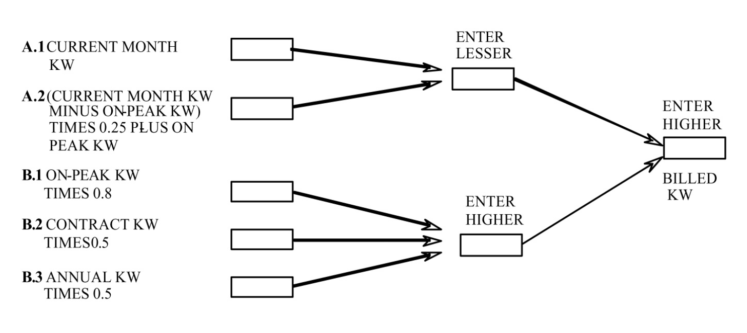
Figure 8-7. Flowchart for the Calculation of Monthly Billing Demand
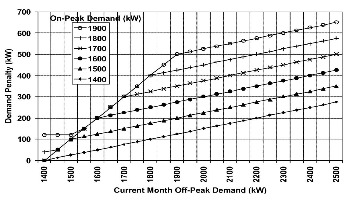
Figure 8-8. Demand Penalties Under Different Current Month Demand Values When On-Peak Demand Has Been Set at Different Levels
Both on-peak and off-peak demand controls are important in minimizing the demand penalty. When the off-peak demand is less than the annual on-peak demand, the demand penalty varies from zero to the difference between on-peak demand and 1,400 kW as the off-peak demand increases to the on-peak value. When the off-peak demand is higher than the annual on-peak demand, the demand penalty is the difference between the on-peak demand and 1,400 kW plus 25% of the off-peak demand increase. For example, if the off-peak demand decreases from 1,700 kW to 1,400 kW when the annual on-peak demand is 1,700 kW, the demand charge will decrease by 300 kW to 1,400 kW. If the annual on-peak demand is 1,400 kW, the demand charge will decrease by 75 kW from 1,475 kW. The demand penalty increases by 75% of the annual on-peak demand increase when the annual on-peak demand is higher than the current off-peak demand.
Figure 8-9 presents a typical storage tank inventory profile, base building electrical load profile (without chillers) and facility electrical load profile during on-peak months. The daily facility electrical load includes the base building electrical power and chiller power. The graphs show a general trend of increased demand from 4:00 a.m. to 2:00 p.m. The base load is 800 kW higher at 2:00 p.m. than at 4:00 a.m. Also note that the demand drops below 1,200 kW after 5:00 p.m. when most staff start to leave the hospital. The base load electrical demand for this hospital is less than 1,400 kW throughout the year, making it possible to set 1,400 kW as the target during off-peak periods.
The chart shows that peak demand is controlled below 1,400 kW. The electrical power is maintained below 2,000 kW until 6:00 am. The off-peak demand is 2,356 kW directly before the on-peak hours.
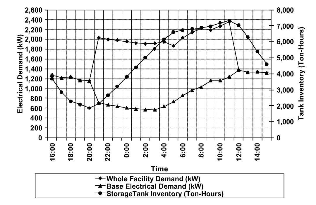
Figure 8-9. Typical On-Peak Months Whole Facility Demand, Base Electrical Demand and Storage Tank Inventory Profiles
The inventory continuously increases after 9:00 a.m. until noon. Obviously, the chiller is charging the tank until noon. If the tank can be fully charged before 9:00 a.m., the off-peak demand can be decreased from 2,350 kW to 2,200 kW. The demand charge will be decreased from 1,650 kW to 1,600 kW with 50 kW demand savings. If the discharging mode could start as early as 7:00 a.m., the off-peak demand can be limited to 2,000 kW. The monthly demand charge can be further decreased from 1,600 kW to 1,550 kW. It appears that the off-peak demand reduction can potentially decrease the demand charge by 100 kW during the summer months.
During winter months, the cooling energy consumption is very low. Most of these buildings were built before 1950. Each room has exterior walls and windows. If the chillers are kept off, the off-peak demand will be below 1,400 kW. Then, 600 kW off-peak demand reduction can be achieved during the winter months since the current control sequence often runs chillers during the daytime. The potential demand charge reduction will be 200 kW for winter months. The demand charge savings varies between 100 kW and 200 kW from summer months to winter months. This is 14% to 28% of design peak load reduction for the thermal storage system.
The peak demand can be controlled at 1,400 kW if the chillers are kept off during the on-peak hours. However, the chillers had to be turned on before the project, which created a peak demand of 1,731 kW. Keeping stable operation means another 250 kW demand charge reduction. It appears that optimizing on-peak and off-peak demand control can decrease the monthly demand charge by 350 kW to 450 kW, which is 50% to 64% of the initial design demand reduction expected from the thermal storage system.
Comprehensive building commissioning was conducted prior to developing the optimal control sequences. During the building commissioning, the AHU operation was optimized. This included static pressure reset, supply air temperature reset, outside air adjustment and other measures. The building chilled water loop was optimized using a loop differential pressure reset. A loop water balance was also conducted in a number of buildings.
The optimized control sequences are discussed separately for on-peak months and off-peak months. A number of factors are incorporated into the sequence to increase the savings and simplify the operation.
On-Peak Months Optimal Control Sequences:
- Turn off one 450-ton chiller at 8:00 a.m.
- Start discharge mode at 9:00 a.m. or later if necessary
- Start the 200-ton chiller at 5:00 p.m. if the inventory is inadequate and the facility load is below 1,200 kW
These sequences are easy to understand and easy to implement. Figure 8-10 compares the measured facility electrical load profiles before and after implementation of the optimized control sequences. The improved control sequences limited the off-peak demand to 2,000 kW by turning off the 450-ton chiller after 8:00 am. Figure 8-10 also shows that commissioning also decreased the facility electrical load significantly.
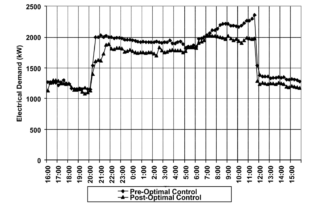
Figure 8-10. Comparison of Typical Facility Electrical Demand Profile Before and After Implementation of Optimal Control Sequences
Optimal Control Sequences for Off-Peak Months
Load projection is critical for the off-peak months optimal control sequence. Cooling load models were developed using measured data as:
The hourly temperature is projected for each day using standard daily profiles combined with forecasted high and low temperatures of the next day. Whole campus cooling load is predicted 24 hours ahead of time to determine the cooling tonnage to be charged. Hourly cooling load up to 5 p.m. of the next day is calculated and totaled every hour after 5 p.m. It is then compared with the cooling capacity remaining in the storage tank.
At 5:00 p.m., the high and low temperature forecasts for the next day are manually entered into the control system. Then the chiller status is determined using the following rule: if the forecast daily cooling is 1,000 ton-hours less than the tank inventory, no chiller will be turned on. Otherwise turn on the chiller and charge the tank until the inventory is 1,500 ton-hours higher than the forecasted cooling load. If the chillers are to be operated, the electrical demand is monitored to make sure that it does not surpass 1,400 kW. If demand drops below 1,000 kW while the 200-ton chiller is in operation and the tank capacity is more than 1,000 ton-hours short, turn on the 425-ton chiller to serve the buildings and charge the tank. If the demand approaches 1,400 kW, turn off the smaller chiller.
The optimal control sequences were implemented in two phases. The first phase, implemented in 1998, focused on controlling the on-peak demand below 1,400 kW. The second phase, implemented in 1999, concentrated on managing the off-peak demand.
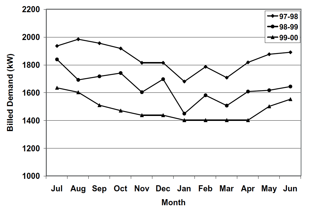
Figure 8-11. Comparison of Billed Electrical Demand Before and After Commissioning
Figure 8-11 compares the demand charges for the base year (1997-1998), after the first phase (1998-1999) and after the second phase (1999-2000). In the base year, the on-peak demand was 1,731 kW and the off-peak demand was 2,736 kW. After the first phase, the on-peak demand was supposed to decrease to 1,400 kW. However, unexpected system failures resulted in an on-peak demand of 1,559 kW. Still, the annual demand charge reduction was 2,215 kW, or 10.0% of the base year demand charge. After the second phase, the on-peak demand was decreased to 1,332 kW. The off-peak demand was controlled between 1,879 kW and 2,207 kW during on-peak months and between 1,318 kW and 1,746 kW during off-peak months. The annual demand charge decreased from 22,158 kW/yr to 18,075 kW/yr for an 18.4% reduction. If the facility were to reduce its contract demand from 2,800 kW to 2,500 kW, it would result in 612 kW of additional demand charge savings. The total potential demand charge savings are 6,910 kW, or 28% of the base year demand charge. More information regarding this case study can be found in “Practical Optimization of Full Thermal Storage Systems Operation” [ Wei et al. 2002].
8.4 Set Up an Alarm System
An alarm system should be in place that will immediately alert the operator if a chiller is accidentally turned off. This will enable the operator to take any actions needed to get the chiller back on line so the tank will be fully charged during the charging period.
References
Liu, M., B. Veteto and D. E. Claridge, 1999. “Rehabilitating A Thermal Storage System Through Commissioning.” ASHRAE Transactions, Vol. 105, Part II, pp. 1134-1139. Wei, G., M. Liu, Y. Sakurai, D.E. Claridge and W.D. Turner, 2002, “Practical Optimization of Full Thermal Storage Systems Operation.” ASHRAE Transactions-Research, Vol. 108, Part II, pp. 360-368.